The Only Retirement Planning Software You’ll Ever Need
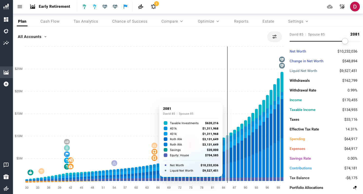
ProjectionLab in action: net worth projections by account type, interactive milestones, tax analytics, stress-testing, and scenario comparison; all in one intuitive dashboard. We walk through everything below.
Reading time: 15 minutes
Advertising disclosure: This article contains affiliate links, marked with an asterisk (*). If you open an account through one of them, The Good Life Journey may earn a commission from the provider, at no extra cost to you. This doesn't influence what we recommend: I use ProjectionLab myself for my own retirement planning, and this walkthrough covers both what it does well and where simpler tools may be enough. More in our full affiliate disclosure.
Quick Answer
ProjectionLab is a retirement planning simulator that lets you model your full financial picture: income, expenses, investments, taxes, Social Security, and major life events. It then allows you to stress-test the whole plan and different what-if scenarios against a century of market history to better understand whether your plan actually holds up.
It’s my favourite retirement planning software in the Financial Independence (FI) space, and allows you to build a solid baseline scenario set in under 15 minutes. Once you start playing with different scenarios—adjusting your retirement age, modeling a move abroad, optimizing taxes, or comparing portfolio withdrawal rates in retirement—it starts to feel more like a fun and intuitive strategy computer game.
What You'll Get From This Article
✔ Full walkthrough of ProjectionLab using a US example: from input data to scenario stress-testing
✔ How to set up your baseline plan in under 15 minutes
✔ How to stress-test your retirement against a century of real market history data
✔ Five scenarios that improve a baseline retirement plan, and what we learn from each optimization
✔ Why tax optimization improves your wealth projection but doesn’t address the most important risk
✔ The one lever that actually addresses sequence-of-returns risk (SORR)
✔ My honest take on who gets the most from it and who might want to wait
TL;DR: ProjectionLab (PL) at a Glance 🧮
🎯 A retirement simulator that models your finances and stress-tests your plans against market history
💰 PL models what simple tools can’t: taxes, Roth conversions, Social Security, withdrawal order & more
🏗️ Layers in life events: mortgage, kids’ education, career changes, rental income, inheritance, healthcare
🎮 Genuinely enjoyable to tinker with. It feels closer to a strategy game than a boring spreadsheet
⏱️ Solid baseline in 10–15 minutes; the deep stress-testing is where you can voluntarily spend hours
🌍 Can model retirement abroad with different expense levels; pairs with geographic arbitrage planning
Why a Simple FI Calculator Isn’t Enough for Retirement Planning
If you’re a regular reader of the blog, you know that I built a Financial Independence Calculator myself for readers to estimate when they could potentially reach early retirement. I still highly recommend it as a first step for anyone who is new to the concept of FIRE (Financial Independence, Retire Early), because it allows you to internalize deep down the importance of your saving rate in reaching Financial Independence (FI) and how retiring abroad could dramatically reduce that timeline.
But this type of tools assume constant stock market returns and spending throughout your whole career, no changing taxes, and no surprises. It gives you a nice entry point to learning about Financial Independence, but it doesn’t reflect the complexity of our financial lives.
In practice, our ability to save and invest changes constantly: childcare costs spike, then disappear; we might work part-time for a few years; a sabbatical or big trip reshapes one year’s budget completely; the mortgage gets paid off or we downsize; an inheritance arrives. A simple calculator treats all of this as a flat line, but, of course, real life is more complex.
We just presented some examples of the complexity of our financial lives during the accumulation side of Financial Independence, i.e., when we are still working. But the early retirement dream also has the post-career period to analyze. For example, would-be early retirees must question what portfolio withdrawal rate they’ll use in retirement and whether it will successfully address sequence-of-returns risk (SORR).
There are also important tax issues to consider as you move away from earning to withdrawing from your portfolio. For instance, from which accounts will you withdraw and in what order? It also presents Social Security timing decisions, variable healthcare costs (potentially increasing in late retirement), perhaps an inheritance or selling a house, or maybe moving to a different country with different costs and tax regimes.
A simple FI calculator gives you a sense of the destination and gives you the motivation to be a more conscious spender. It allows you to better understand the trade-offs between consuming less now and retiring earlier in the future. But it doesn’t tell you whether your individual pathway to FI is survivable in practice.
That’s the gap ProjectionLab fills. PL lets you model the full complexity of your financial life and stress-test whether your plan holds up even when markets are not cooperating.
What made me personally move from step 1 (using a simple FI Calculator) to step 2 (a more complex software) was a simple frustration: I write a lot on this blog about safe withdrawal rates in retirement, sequence-of-returns risk (SORR), variable spending strategies, or the impact of geographic arbitrage on your FI timeline. But generally I tend to consider all of these issues separately in different analyses, while in reality all of these different aspects of the FI journey interact with each other.
And that is by far what I appreciate most about ProjectionLab. Having it all in a single model that you can edit and re-run with one click is really helpful. I can run “what-if simulations” on my plan and try to change my withdrawal rate over a limited period, and see what happens. Or decide to move abroad a few years for an early retirement adventure, and see what happens. Whatever life change you’re considering, you can see in a few clicks how it affects your portfolio’s survivability.
Other examples that are useful in my situation: modeling my kids’ eventual college costs, or how our recent decision to take an extra full month of unpaid leave each year affects our FI timeline. We also currently pay a fairly expensive rent in a mid-sized city, but may buy or rent somewhere cheaper at some point in the future. Yet another layer of complexity the model can handle easily.
Recently, a friend of mine tried using our FI calculator and said something along the lines of: “I really appreciate the calculator to get a rough idea of my timeline, but I have many moving parts in my life at the moment”. Indeed, he’s currently paying a fortune for his toddlers’ kindergarten, but this cost will disappear soon; he’s in a high-stress, high-pay role now, but thinks he won’t hold on to it for long and may take a lower paying job soon; he’s considering buying a second property but doesn’t fully understand how it affects his ability to retire early. All of this complexity can be modeled easily in PL with a couple of clicks.
The Case Study: Setting Up a Retirement Plan in 15 Minutes
Meet the example household
Let’s walk through the tool with a realistic example. The numbers are made up, but the process is exactly what you’d follow with your own, so it’s worth going all the way through.
The household’s finances we want to model are from a US-based couple, both 30, living in Denver, Colorado. Each earns $70,000 per year; a combined gross income of $140,000. That’s not too far away from what median salaries look like in the US.
The couple discovered Financial Independence (FI) a few years ago and have been saving consistently ever since, though they’re still building up their emergency fund and paying off student loans. Between both of them they have $365,000 in net worth. As we’ll see, their wealth is scattered across retirement accounts, brokerages, and real estate.
In Figure 1 and immediately below we present the full breakdown:
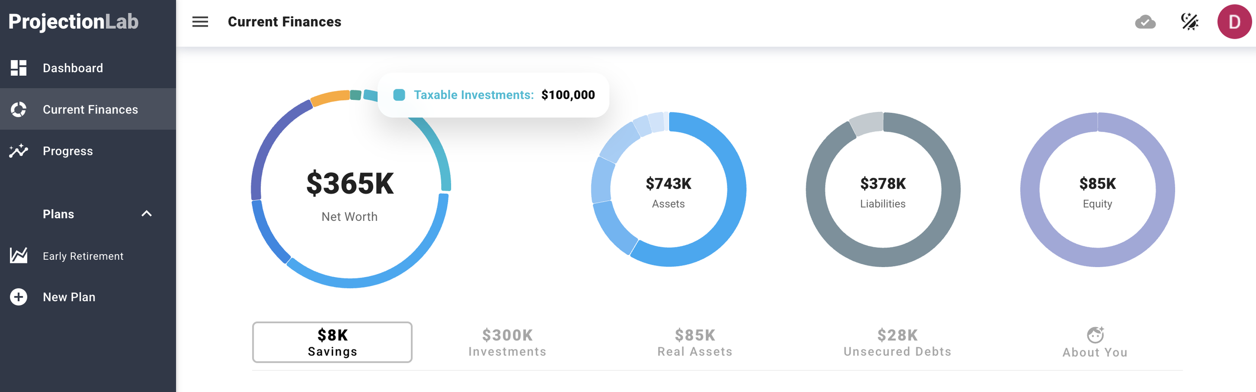
Figure 1: High-level breakdown of current finances of our US household. In ProjectionLab, user can click each component of the donut to explore further.
Investments ($300,000): $150,000 in 401(k) accounts ($75,000 each, with each person contributing 6% of salary and their employers matching half of that), $50,000 in Roth IRAs (again, $25,000 each, each contributing the $7,000 annual maximum), and $100,000 in a joint taxable brokerage account.
Savings: $8,000 in a high-yield savings account. This is clearly underfunded at the moment; their goal is to build up their cash reserves slowly to $20,000.
Real assets: Their home is valued at $435,000, purchased three years ago for $420,000 with a 10% down payment. Current mortgage balance is $350,000 at 6.5% on a 30-year fixed, with monthly payments of about $2,400.
Debts: the mortgage mentioned above plus student loans ($28,000 combined, at 5.5% annual percentage rate, with $600/month in payments).
Net worth: all this considered their net worth is $365,000. Of course, this number is slightly deceptive in relation to FI because $85,000 is illiquid and tied to their house.
Their goal: reach Financial Independence as soon as possible, possibly live temporarily abroad.
The savings flow, and why the order matters
ProjectionLab asks early on to prioritize where your money goes, and that order matters, because it tells the software how to allocate income flows of money. This is what we set in our example, from top priority to bottom:
401(k) to the employer match (6%). This is free money; the employer match is a guaranteed 50% return on your contribution. There are not many times in life when you get such a guaranteed return on your money, so be sure to take it.
Emergency fund to $20,000. Their current $8,000 cash reserves are pretty thin relative to their expenses (more on this later). We want to make sure we build our cash reserves first before accelerating investments.
Roth IRA to the annual max ($7,000 each). This is after-tax money going into investment accounts that are allowed to grow tax-free forever. Roth IRA can be withdrawn anytime without penalties (unlike 401(k)).
Taxable brokerage with everything remaining. Here there are no tax advantages, but, of course, it’s fully liquid with no age restrictions or withdrawal penalties.
It’s important to note something we didn’t add: we chose not to layer on extra payments on the student loans or mortgage. At 5.5% (student loans) and 6.5% (mortgage), the “return” from paying off debt faster is lower than the long-term expected ~7% from investing. The math would flip if these debts were at 8%+, but at these rates, investing the difference is likely to come out ahead over time.
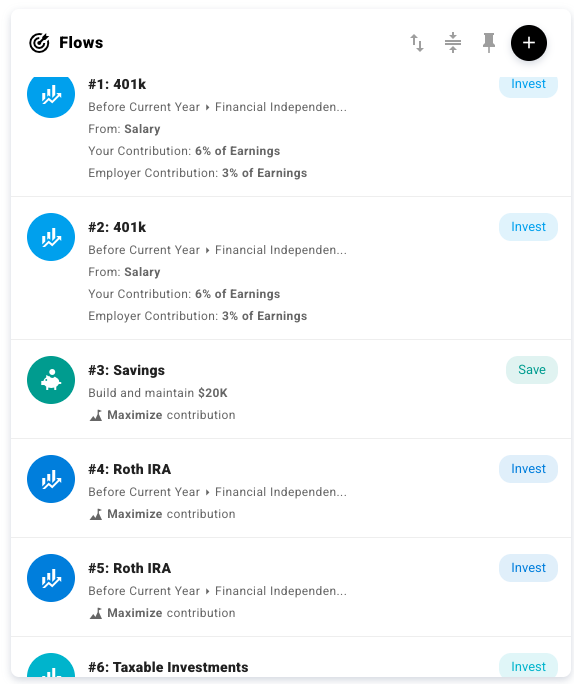
Figure 2: ProjectionLab allocates your income top to bottom: each dollar flows to the highest-priority account first, in this case 401(k), and only what’s left moves to the next.
Setting Milestones: sketching the shape of your financial plan
This is where ProjectionLab feels very different from a simple calculator. Instead of assuming one straight line from now to death, you start by defining the major transition moments that shape your plan. A milestone can be anything: reaching FI, a career change, a move abroad, a child’s birth, a house sale, or a shift in spending.
Input data you enter like income, expenses, investment contributions, and withdrawals can all be tied to specific milestones or periods between them rather than hardcoded to ages, so when you later run scenarios where you ask “what if I retire two years earlier?” the entire plan adjusts automatically.
In our simplified example, we set the following milestones:
Retirement at Financial Independence. So our working phase goes from age 30 to FI. But you could set it differently, e.g., work a few years after reaching FI.
Financial Independence: PL triggers this when liquid assets reach x times annual retirement expenses. In our example we set x20, which is effectively a 5% withdrawal rate.
Post-FI: earned income stops, general living expenses drop slightly by $5,000 (no commuting, no work lunches, no work-related or stress-related consumption, more time to cook, etc.). We’re modeling the same quality of life with a slightly lower spend.
In addition to the milestones you enter yourself, PL generates another set of indirect milestones that reflect your situation. In our case study, for example, the chart displays also the following milestones:
When the emergency fund is fully funded
The student loans are paid
Start of slightly lower discretionary expenses in retirement
Start of medical expenses in early retirement
The house mortgage is fully paid
Start of Medicare
All the milestones appear interactively on the chart, so you can click to examine them and edit as needed. The whole set up, including entering basic information, milestones, income, expenses, etc. takes 10-15 minutes. And already here, before stress-testing and further optimizing your plan, ProjectionLab already generates a very useful baseline.
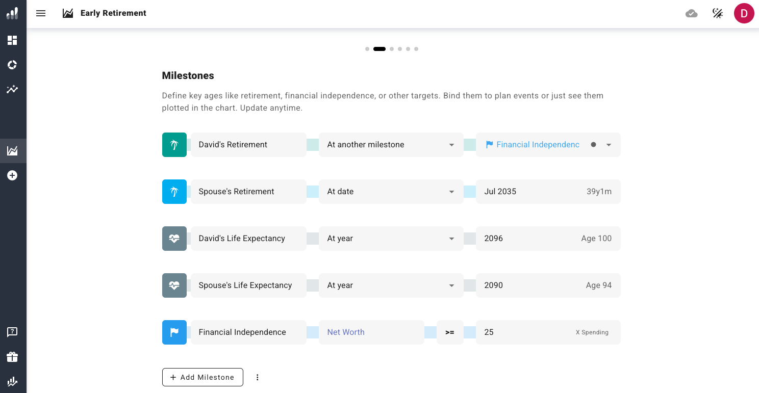
Figure 3: Definition of milestones. In this case, moment of retirement, life expectancy, and definition of Financial Independence. Screenshot shows x25, but we actually ended up using x20 (a 5% SWR). We also set spouse’s life expectancy to 100.
The Baseline Results, Before Any Stress-Testing
The baseline projection: a first look at the full picture
With all the inputs in place, ProjectionLab generates the baseline scenario shown in Figure 4 below. This is the projected trajectory of the couple’s net worth, broken down by account type. Importantly, this figure is assuming constant, average market returns. But as we’ll explore in further sections, the order in which these returns happen matters much more than the average you end up getting over a given period.
Several things stand out immediately. The net worth in the early years picks up slowly; that’s not only because part of their income goes to funding the emergency fund and to paying student and housing loans. It’s also due to compounding; the effect becomes more clear the more years pass.
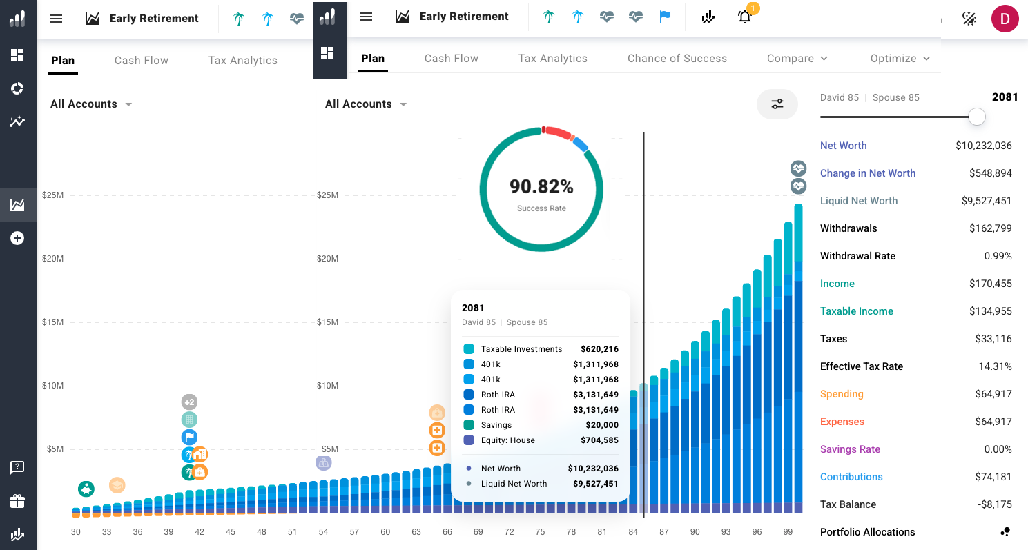
But around their mid 40s, and especially after paying off their house, the compounding starts to visibly take over. By age 85, and assuming their lifestyle hasn’t changed over time, their net worth reaches about $10M in today’s dollars, out of which $9.5M is liquid. The Roth IRA accounts dominate the later decades, which makes sense: they’ve been compounding untouched and tax-free for over 50 years by that point. As we’ll see later, PL correctly prioritizes withdrawing in retirement from other accounts first.
The interactive graph (see screenshot below) lets you hover over any year and see the exact breakdown: how much sits in each 401(k), each Roth, the taxable brokerage, savings, and home equity. As mentioned, you can also click and edit the milestone icons displayed on the chart.
Here’s a quick overview of what’s visible on the chart (Figure 4): emergency fund fully funded by age 32 (year 2), student loans paid off by 34 (year 5), Financial Independence reached at 41 (year 12). At this point both partners retire, earned income stops, and slightly lower post-FI living expenses kick in (but also new healthcare costs). The mortgage is fully paid off by 54, and Medicare replaces their private healthcare costs at 65.
Of course, this is a single projection assuming average returns. It’s the rosy version, but we shouldn’t be fooled by it. The stress-test in further sections will show us how this plan performs when markets don’t cooperate, i.e., if you’re unlucky enough to have 2-3 consecutive poor-return years in early retirement.
But before we get there, this baseline projection (labelled as “Plan” in PL) already reveals three important insights that we might have missed with a simpler tool.
Figure 4: Baseline scenario. Projected net worth by account type, assuming average market returns. Key milestones visible on the timeline include student loan payoff (paid off in year 5), emergency fund fully funded (year 2), Financial Independence (year 12 at age ~41), retirement, and mortgage payoff (age 54). The Roth IRAs (dark blue) dominate the later years thanks to decades of untouched tax-free compounding. Important caveat: this is a single projection using average returns. It’s not giving the full range of possible outcomes. The stress-test (Chance of Success tab, covered further below) reveals how this plan really performs across different historical market periods, giving you a far more useful datapoint.
👉 Want to build your own baseline? You can set one up in under 15 minutes. Check out ProjectionLab with their 7-day free trial to get a sense of whether it’s worth paying to unlock its full functionalities:
Three things we learned before running any simulation
Our first insight is regarding the savings rate, the single most important factor determining the speed of FI. In our case study it isn’t constant over time, as is often assumed in other tools. At age 30, ProjectionLab shows an effective rate of about 27% (Figure 5 below). But by the time the student loans are paid off around age 34, it jumps to 35%, without any changes in lifestyle. This ties back to the point we made earlier with my friend. Life is messy, and savings rates tend to go up and down over time.
Once the loan payments are gone, the $7,200/year redirects entirely to investments. PL shows this automatically; a simple calculator would assume a flat savings rate over the whole period.
Second, the couple made it to FI in only 12 years on a savings rate that never exceeded 38%. Granted, they started out with some savings and investments, but it’s far from being a Silicon Valley story. It’s a dual-income household earning roughly the US median. Taking advantage of the employer match and compounding on the existing $300,000 is doing a lot of the work here.
Third, Financial Independence based on net worth and FI based on liquid assets results in different early retirement dates. When we initially set the FI milestone to trigger on x20 total net worth (including the house), PL said they were FI earlier, but then had to implement very high withdrawal rates from their portfolio—close to 6%. This didn’t provide solid results when stress-testing the plan against market history data.
The house represented a relevant share of their net worth by then, but you can’t live off home equity. Switching the milestone trigger to liquid assets instead only pushed the FI date back by a few years, but the withdrawal rate started at a much healthier level (the targeted 5%). This is yet another subtle but critical distinction that may have been overlooked by a simple calculator. In contrast, when you run portfolio survival tests on the first definition you realize very quickly there is something wrong with your plan.
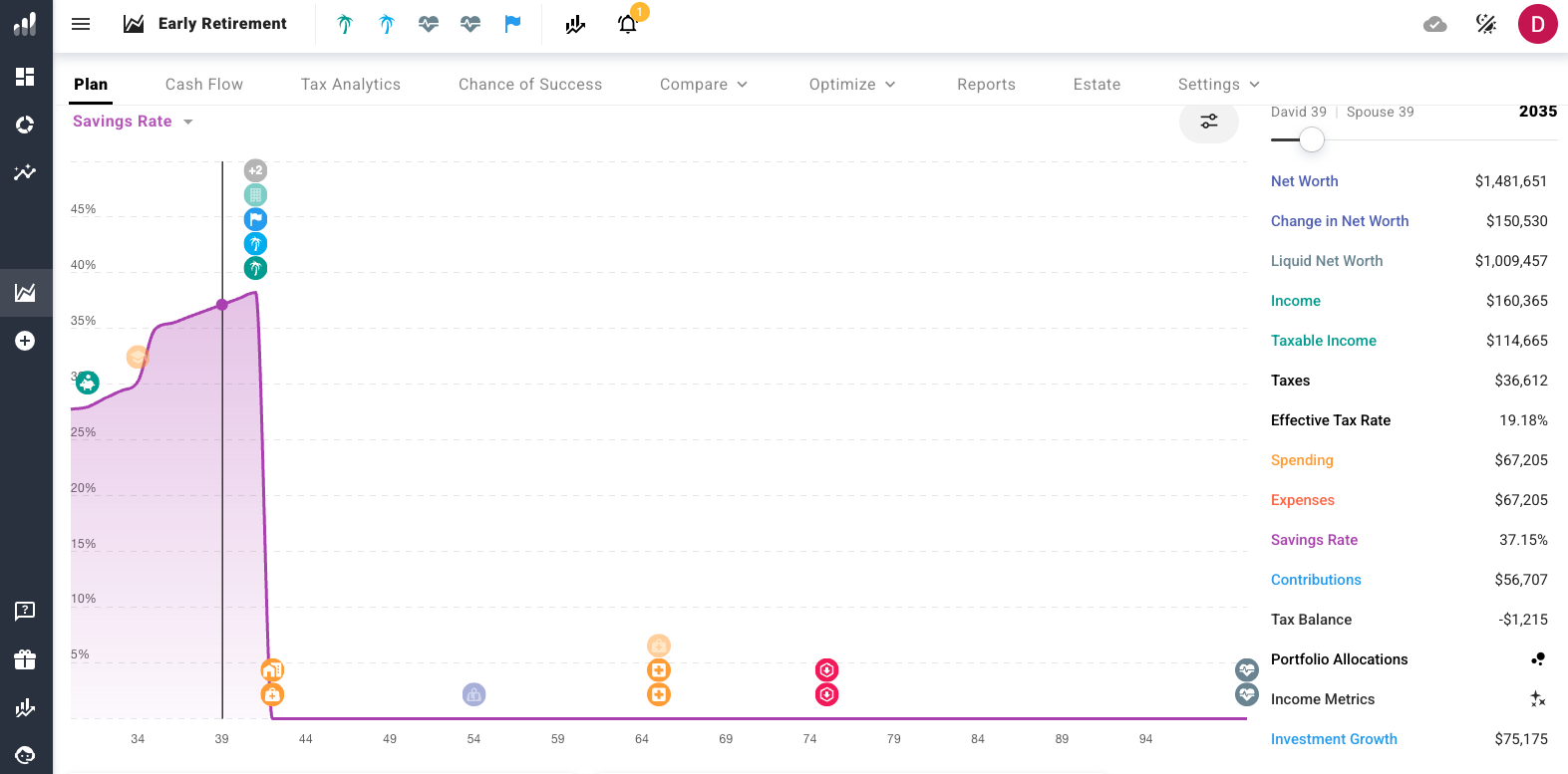
Figure 5: Savings rate over time. As observed, the 12-year timeline to FI goes from a 27% savings rate to a 38% right before FI. The numbers displayed on the right are for 2035. You can click any year on the graph to see the year-specific data. You can also click on those elements (e.g., income, taxes, etc.) to get a more detailed breakdown.
The withdrawal order: where your money comes from
One of ProjectionLab’s most compelling features is understanding each individual’s tax picture and prioritizing which accounts to withdraw from in early retirement. I’m not a tax expert and I’m based in Germany, but it’s incredible how much I’ve learned about US taxes after playing around with PL with a US example.
For our case study baseline (before further optimization), the order of withdrawal would be as follows (Figure 6):
Ages 42–54: taxable brokerage. PL draws from this first because there are no age restrictions or penalties, just capital gains tax on the profit portion of what is sold. This is the bridge account that early retirees need before they can tap into other tax-advantaged accounts.
Ages 54–59: 401(k) with penalties. Once the brokerage runs dry, PL taps into the 401(k). But since we’re withdrawing under age 59½, every withdrawal gets hit with a 10% early withdrawal penalty on top of income tax. This shows up as a warning in PL: a yellow bell on the dashboard, but also the bar chart is colored red and labeled as “penalized distributions.” We’ll come back to how to optimize this in further sections below.
Ages 60–74: 401(k) penalty-free. Past 59½, the penalty disappears and you can withdraw from your 401(k) without penalty.
Ages 75+: 401(k) forced withdrawals (Required Minimum Distributions or RMDs). Starting at 75, the IRS requires you to withdraw a minimum amount from tax-deferred accounts each year. In our case study, and assuming average returns, the 401(k) is large enough to cover spending entirely on its own. The Roth IRAs are never tapped and simply keep compounding tax-free as a legacy asset in this pre-optimization, baseline scenario.
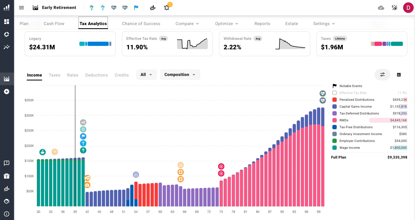
Figure 6: The full tax picture before any optimization: income sources across a lifetime in one chart. During working years (green), salary dominates. After retirement, the brokerage bridges the gap (purple), then 401(k) withdrawals take over. First, with penalties (red), then penalty-free, then as forced RMDs (pink) that grow into a wall from age 75 onwards. Notice how PL is highlighting in red $4.8M in lifetime RMDs and an 11.9% effective tax rate. We’ll fix this in the next section.
Two main issues stand out from this chart. First, the red penalty window in the mid-50s, which is money lost to a 10% surcharge simply because of poor withdrawal timing. Second, look at the shape overall: we have modest withdrawals early on in retirement, then a large wave of forced RMDs from age 75 onwards, growing larger every year. Clearly, as we’ll see in a later section, there is room here to further optimize the withdrawal order and associated taxes we end up paying.
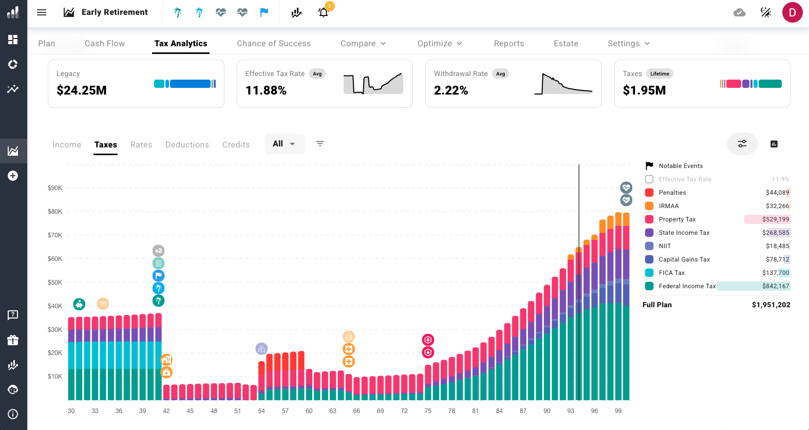
Figure 7: Lifetime taxes broken down by type—$1.95M total (modeled until age 100). Federal income tax (green) and property tax (pink) are the two largest components, but notice the red penalty bar in the mid-50s and the ballooning taxes from age 75 as RMDs force increasingly large taxable withdrawals. PL lets you click any individual year to see the exact breakdown.
Stress-Testing Your Retirement Plan Against Real Market History
Everything so far was a projection assuming constant average returns every year (7% real return). But as we’ve covered many times in the blog, returns are never consistently average. The order of yearly returns—captured by the concept sequence-of-returns risk (SORR)—matters more than the actual average you end up getting.
If you’re unlucky enough to experience, say, a 30% market drop in your first year of retirement it can be far more devastating than experiencing the same event in year 12 of early retirement. In year two, you’d be withdrawing from a beaten-down portfolio, and that early damage compounds forward in subsequent years. In contrast, if it occurs in year 15, your portfolio has likely grown well beyond its starting point and can absorb the hit much better. Again, same average return over the full period, but dramatically different outcomes depending on when the bad years landed.
ProjectionLab runs your plan against every historical period in its dataset (going back to 1928) and shows you in what percentage of those historical periods your money would have lasted.
The baseline result
For our case study—FI at age 42, with a 5% withdrawal rate on liquid assets—the survival rate comes in at 79–91%, depending on the simulation method used. PL offers many, but here we use the two main ones suggested: a historical random restart (walks through actual historical sequences) and a historical block bootstrap (more conservative, stitches random 5-year blocks).
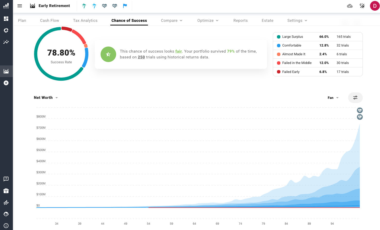
Figure 8: Chance of Success of the baseline scenario, using the historical block bootstrap method (one of PL’s more conservative simulation approaches). The plan survives in 79% of 250 trials. Two-thirds of scenarios end with a large surplus, but nearly 19% fail, either early or mid-retirement.
Is this good enough? Well, to a great extent it depends on your risk tolerance, but many folks (and financial planners) may feel uncomfortable seeing a large range below 90%. This plan would work in the majority of scenarios but is certainly not bulletproof.
The failed scenarios: what goes wrong?
ProjectionLab doesn’t just give you a percentage of success when you stress-test your plan. It also returns exactly which historical periods would have failed, so you can better understand why. Many failures involve a major market downturn hitting in the first 5–7 years of retirement, but also the interplay or poor returns during eras of inflation or stagflation can be a major killer.
Usually, the first 5–7 years of retirement are make-or-break. If you “survive” that window with your portfolio reasonably intact, your withdrawal math is almost certainly going to be fine for life. But if you’re hit with poor returns early on, it’s far from clear whether your portfolio will survive another few decades.
Figure 9 shows one of the failed trials in detail. The simulation maps to the 1955–1989 historical sequence: our couple retires at 41 in 1966, and by age 64 they’re out of money. The damage comes from four double-digit market drops in the first nine years of retirement, made worse by the brutal inflation of the mid-1970s. That’s a combination that portfolios withdrawing at 5% will find very difficult to survive.
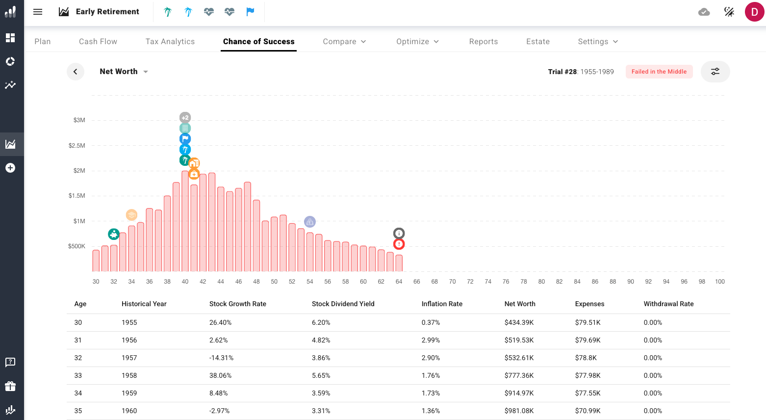
Figure 9: A closer look at one of the failed trials: trial #28, mapped to the 1955–1989 historical sequence. The portfolio peaks around the FI milestone, then steadily bleeds out over the next 25 years, hitting zero by age 64. By then your remaining net worth is your house equity.
Five Ways to Improve Your Retirement Plan’s Survival Rate
Now that we understand our baseline scenario, let’s test five different levers to further optimize our plan, both in terms of the chances of success and the potential for a larger portfolio.
Lever 1: Tax optimization improves wealth, doesn't fix survival
ProjectionLab has a remarkable feature: it provides an automatic tax strategy comparison table that tests every major tax optimization approach against your individual plan in one screen (Figure 10). For our case study, the winner was “Convert and shield to 22%,” which means converting 401(k) money to Roth during the low-income retirement years, capping conversions at the 22% tax bracket.
The logic of these conversions is simple: in the years between retiring and Social Security kicking in, your taxable income is very low, so you deliberately move money out of the 401(k) and into the Roth while you’re in a low tax bracket, rather than waiting for the IRS to force it out later via RMDs at a much higher rate (what we covered previously in Figure 6 and 7 above).
If all this tax talk sounds complex, don’t worry. Scan quickly and move on. Just be reassured that the software allows you to optimize in a couple of clicks your tax situation to avoid overpaying. You’ll be saving money that is many orders of magnitude larger than what PL costs.
By choosing the strategy “Convert and shield to 22%,” PL eliminates $4.8M in forced RMDs over the time period considered and cuts the effective tax rate from 11.9% to 4.6%.
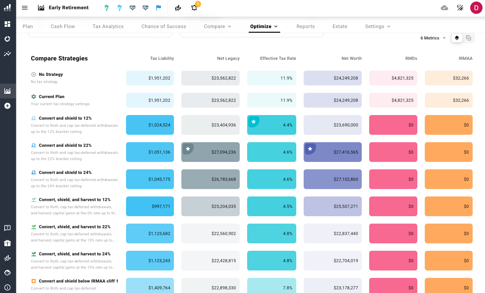
Figure 10: ProjectionLab’s tax strategy comparison table, including every major optimization approach tested against your individual plan in one click. In our case study, the best strategy (“Convert and shield to 22%”) eliminates $4.8M in forced RMDs, cuts the effective tax rate from 11.9% to 4.6%, and increases net legacy in the baseline scenario from $23.6M to $27.1M.
Granted, the net worth numbers provided here are at age 100, so there is extraordinarily strong compounding taking place. But even looking at the portfolio at age 85, net worth goes from $10.2M in the baseline scenario to 10.9M after the tax optimization to avoid the RMDs. We’re talking about a portfolio increase of over $700k.
But while the tax optimization dramatically affects your portfolio and net worth, the survival rate we obtain by assessing historical market returns barely moved, only by about 1%. The reason is that the scenarios that make the whole plan fail are the ones where bad markets hit in the 1-7 first years of retirement, and these tax optimizations don’t affect these earlier years so much. It just rearranges which accounts the money comes from.
The bottom line is tax optimization builds wealth—it makes the good scenarios even better—but it doesn’t fix the scenarios that fail. It’s certainly worth doing, but we need to look elsewhere to address the sequence-of-returns risk.
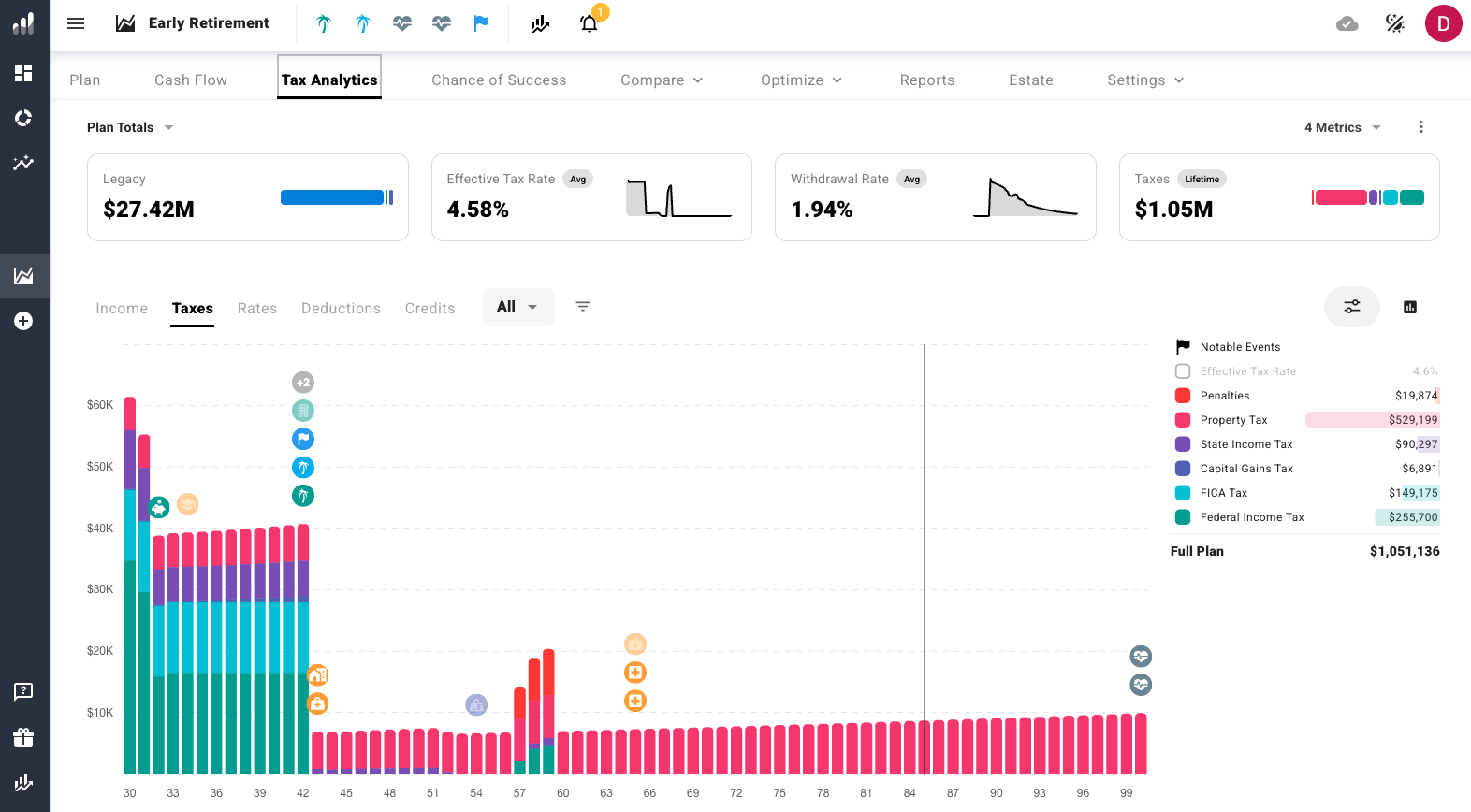
Figure 11: Tax picture after applying the “Convert and shield to 22%” strategy. The massive RMD wall from our baseline scenario (Figure 7) is gone entirely. Lifetime taxes drop from $1.95M to $1.05M, effective tax rate from 11.9% to 4.6%, and the remaining tax burden is almost entirely property tax (pink).
Lever 2: Flexible spending is helpful but modest
We improved our taxes, but the survival rate of our simulations remains largely the same.
Next, let’s introduce some spending flexibility in our withdrawals. Aligning our spending partially with market returns should in theory improve PL’s stress-testing outcomes.
We set 20% of post-FI living expenses as discretionary (excluding housing-related expenses) and set the following rule: if markets drop 10%+, cut that discretionary spending entirely. That’s about $4,400 less per year during downturns: perhaps skipping some travel, eating out less, and tightening the belt a bit when markets are not cooperating.
The surprising result is that it only improves the success outcomes by about 1%. It’s certainly better than not paying attention at all, but at the spending level of our case study, the discretionary slice is simply too small to materially change the outcome.
A household spending $80,000/year with 40% discretionary would see a much bigger impact from flexible spending. For our couple at $22,000 in living expenses (again, not including housing costs), there’s not much left to cut. As observed in the Sankey diagram of Figure 12 below, this household has about $80,000 going in at age 45 (year 3 of retirement), but a lot of fixed costs (mortgage, medical expenses, and house).
The $4,400 in flexibility represents about 5% of their overall budget, so it’s not surprising that for our case study the flexibility lever was not very important in improving the chances of success in our stress test.
Flexible spending can be important, but the magnitude depends on how much of your budget is genuinely discretionary. Don’t overestimate how much you can actually cut when times get tough; there are many items that are hard to budge.
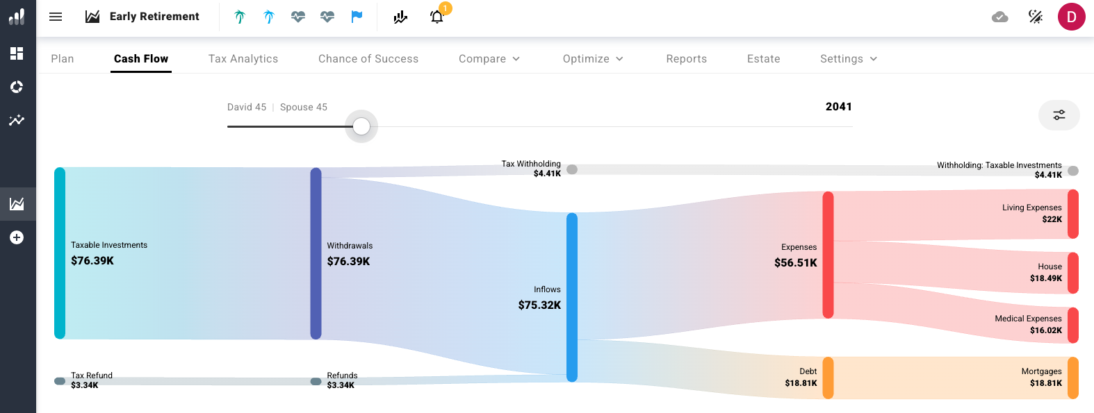
Figure 12: Cash flow three years into retirement at age 45. The Sankey diagram makes the problem visible: of the $75K flowing in, over $53K goes to fixed costs (mortgage, medical expenses, house) that simply can’t flex. The $22K in living expenses is the only adjustable slice, and cutting 20% of that yields just $4,400. It’s barely a dent in the overall picture. PL allows you to click in every year of the plan to see how the cash flow changes over time.
Lever 3: Five years abroad — the SORR fix
We still need to find a way of improving our portfolio’s chances of success into something slightly more acceptable. Let’s suppose that our case study couple decides, upon reaching Financial Independence, to rent out their Denver house and spend five years slow-traveling throughout SE Asia—Thailand, Vietnam, Malaysia—something they’ve always dreamed about doing (and a financially powerful move, as we’ve covered on our article on geoarbitrage). Let’s conservatively keep their same $22,000 annual living expenses, which is their annual budget for living in these low cost-of-living countries.
The rental income they would now receive of $28,800/year roughly matches the mortgage payment, cutting portfolio withdrawals by more than a third during the five years when sequence-of-returns risk is most dangerous.
When we run again the “Chances of Success” simulation on this scenario, the results improve substantially: we go from a 79–91% range in the baseline scenario to 85-98%. Again the upper value of these ranges is considering rolling historical periods, so a plan that would have survived in 98% of past history is very solid. The lower conservative value was using 5-year historical blocks, mixed randomly.
The reason why this notably improves our plan is because it reduced the portfolio withdrawal rate during the exact window where SORR is deadliest: those first 5-7 years of retirement when a market crash can permanently damage your portfolio.
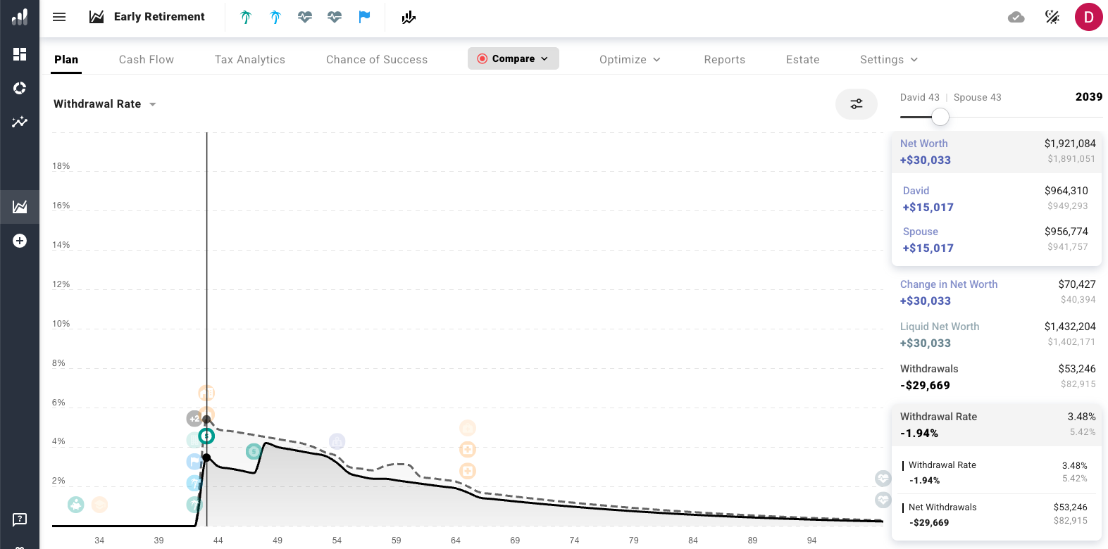
Figure 13: Withdrawal rate comparison of baseline (dashed) vs. five-years-abroad scenario (solid). The rental income drops the withdrawal rate from 5.4% to 3.5% in year one of retirement, and the gap persists well beyond the five-year abroad window.
Lever 4: Adjusting the withdrawal rate
This is the simplest lever of all: what if they targeted a 4.5% withdrawal rate instead of 5%, meaning working slightly longer to build a larger portfolio? Even a small reduction in the withdrawal rate produces a disproportionate improvement in survival because it reduces withdrawals in every year, including the critical early ones. In this case, it improves success from our baseline of 79–91% to 84-98%.
The downside is that it would delay Financial Independence and retirement by about 1 year, but the improvement in peace of mind may be well worth it, especially if other levers like geoarbitrage or spending flexibility are not considered to protect the withdrawal rate in the first years of early retirement.
What We Learned: The Levers That Actually Work
In the table below we summarize the different scenarios we considered:
| Scenario | Success rate | Key insight |
|---|---|---|
| Baseline (5% SWR, stay in Denver) | 79–91% | Workable but not bulletproof |
| Tax optimization (Convert & shield 22%) | 80–92% | Improves wealth dramatically on average return projection, but barely moves portfolio survival when considering real world sequence of returns |
| Flexible spending aligned with market returns | 81–93% | Very modest help in this example, but can make an important difference in budgets with a lot of discretionary spending |
| Five years abroad (rental income, lower withdrawals) | 85–98% | The big lever — directly attacks SORR |
| Lower withdrawal rate (4.5% instead of 5%) | 84–98% | One more year of work buys significant peace of mind |
Sequence-of-returns risk (SORR) is the real enemy of early retirement, and levers that reduce withdrawals during the first 7 years or so meaningfully improve your odds. Tax optimization, while very important and worth potentially hundreds of thousands in lifetime wealth, barely touches the failure scenarios.
Flexible spending helps but is limited by how much of your budget is genuinely discretionary. Geographic arbitrage—spending the riskiest early years in a lower cost-of-living location—turned out to be the lever that actually moved the needle on portfolio survival. Of course, this is because we targeted a FI number of x20 times our expenses (a 5% withdrawal rate). Aiming for a more conservative withdrawal rate (and a larger initial portfolio) also reduces risk considerably.
A few caveats worth stating explicitly. These results we presented are specific to our case study; a US-based couple with a 5% withdrawal rate, a mortgage, and a particular account mix. Your specific situation will produce different outcomes, and that’s the whole point of running your own plan. The scenarios we tested are also not exhaustive. PL can model far more than we showed here. What is transferable is the process itself: build a baseline, stress-test it from different angles, and systematically test the levers that move the needle for your situation.
Other Features Worth Exploring
This walkthrough focused on the scenarios most relevant to our case study, but PL can model far more than what we showed. Some other features worth exploring once your baseline is set up:
Life event modeling: People’s income and expenses change a lot over time. Consider kids’ education, career changes, inheritance, house purchases and sales, sabbaticals, or one-off large expenses. In PL, each is just another event on the timeline. As I mentioned earlier, being able to layer in variable expenses like kids’ university costs now alongside near-term childcare expenses gives me a level of clarity that free FI calculators simply can’t provide.
Portfolio allocation over time: You can enter different stock-to-bond allocations and even design desired glide paths and see how they perform. You can also add a bond tent to handle SORR. The ability to test how different stock/bond mixes affect both your timeline to FI and your survival rate in retirement is powerful.
Withdrawal strategy comparison: fixed 4-5% vs. guardrails vs. other strategies compared side by side on your actual numbers.
Estate planning: PL has a dedicated Estate tab that models what you leave behind, including how different tax strategies affect legacy wealth.
Is ProjectionLab Worth $129 Per Year?
Let’s try to put that number in context. In our case study, the tax optimization alone—a few clicks in PL’s strategy comparison table—saved hundreds of thousands in lifetime taxes and increased the projected net worth by $700,000 at age 85. The tool paid for itself roughly 5,000 times over in the very first scenario we tested. (Note: $129 is the base price; depending on your location, VAT or sales tax may apply on top, though we’re talking about a few extra dollars.)
Setting aside the extreme compounding of a 60-year projection, the practical value is harder to quantify but arguably more important: the peace of mind that comes from knowing your optimized plan could have survived the Great Depression, the 1970s stagflation, the dot-com crash, or the 2008 financial crisis. The future is always uncertain, but being as prepared as possible is definitely a good move.
I think most people reading this blog would get genuine value from using ProjectionLab. Our real-world financial lives are more complex than we think: we need to consider different account types, a mortgage, a potential relocation, kids, different retirement timelines for each spouse, Social Security timing decisions, other changing income or expenses over time, questions about withdrawal strategies, etc.
PL turns all that noise into a single model that allows us to stress-test and adjust our plan in real time. Your retirement is the biggest financial decision you’ll ever make. Stress-testing it from different angles costs $129 a year. As we’ve illustrated here, not optimizing your plan or failing to stress-test this can literally cost you many hundreds of thousands of dollars, or worse, discovering that your plan doesn’t hold up at all.
The only group I’d point elsewhere first are those who are completely new to Financial Independence and haven’t yet calculated their own FI number or don’t yet understand at a basic level how their savings rates drive their FI timeline. For those, I’d start with the free FI Calculator. But if you’re already comfortable with the concept of FI, using ProjectionLab is the obvious next step.
If you’ve read this far, you already know whether your own plan has the kind of complexity that deserves stress-testing. If you’re still unconvinced, ProjectionLab offers a 7-day free trial: enough time to build your baseline, play around with the features, and see for yourself whether unlocking its full functionality is worth roughly $15 per month.
If you found this walkthrough useful, here are a few related resources:
👉 New to FIRE? Start with our Complete Financial Independence Guide
👉 Deep dive into withdrawal strategies: Safe Withdrawal Rates Explained
👉 Considering retiring abroad? Geographic Arbitrage & FIRE: The Complete Guide
👉 Model where to retire across 100+ countries: our free Retirement Relocation Tool (email unlock)
🌿 Thanks for reading The Good Life Journey. I share weekly insights on personal finance, financial independence (FIRE), and long-term investing — with work, health, and philosophy explored through the FI lens.
Disclaimer: I am not a financial or legal adviser, and this content is for informational and educational purposes only. Please consult a qualified financial adviser for personalized advice tailored to your situation.
Check out other recent articles





























About the author:
Written by David, a former academic scientist with a PhD and over a decade of experience in data analysis, modeling, and market-based financial systems, including work related to carbon markets. I apply a research-driven, evidence-based approach to personal finance and FIRE, focusing on long-term investing, retirement planning, and financial decision-making under uncertainty.
This site documents my own journey toward financial independence, with related topics like work, health, and philosophy explored through a financial independence lens, as they influence saving, investing, and retirement planning decisions.
Frequently Asked Questions (FAQs)
-
ProjectionLab is a retirement planning simulator that lets you model your full financial picture — income, expenses, investments, taxes, and major life events — then stress-test the entire plan against nearly a century of real market data. It shows you in what percentage of historical periods your money would have lasted, giving you a far more realistic picture than any single-number FI calculator.
-
For anyone with meaningful financial complexity — different account types, a mortgage, kids, potential relocation, or questions about withdrawal strategies — the value is substantial. In our case study walkthrough, a single tax optimization that took two clicks saved over $700,000 in projected net worth by age 85. The tool pays for itself many thousands of times over if it helps you make even one better decision about withdrawals, tax timing, or retirement timing.
-
Sequence-of-returns risk (SORR) is the fact that when bad market years hit matters far more than your average returns over time. A 30% market drop in your first year of retirement is devastating because you’re withdrawing from a shrunken portfolio, and that early damage compounds forward. The same drop in year 15 matters less. SORR is the single biggest threat to early retirement plans and the primary reason stress-testing tools like ProjectionLab exist.
-
Yes — it’s one of the tool's strongest features. PL provides an automatic strategy comparison table that tests every major approach (Roth conversions at different tax brackets, capital gains harvesting, RMD avoidance) against your specific plan. In our case study, the optimal tax strategy eliminated $4.8M in forced Required Minimum Distributions and cut the lifetime effective tax rate from 11.9% to 4.6%.
-
Spending the first years of retirement in a lower-cost country reduces portfolio withdrawals during the exact window when sequence-of-returns risk is most dangerous. In our case study, renting out a Denver house and spending five years in Southeast Asia at the same lifestyle budget improved the plan’s historical survival rate from 79–91% to 85–98% — far more than tax optimization or flexible spending achieved.
-
The classic answer is 4% (the “4% rule”), meaning you withdraw 4% of your portfolio annually. However, recent research suggests rates between 4% and 5% may be sustainable depending on flexibility, time horizon, and other income sources. The key insight from stress-testing is that the “safe” rate depends heavily on your specific plan — account types, tax situation, spending flexibility, and whether you have strategies to reduce withdrawals during market downturns.
-
A simple FI calculator tells you when you’ll reach Financial Independence based on fixed assumptions — constant returns, constant spending, no taxes. ProjectionLab models your full financial complexity (multiple account types, changing expenses, tax brackets, life events) and then stress-tests the plan against real historical market data. Think of the calculator as showing your rough destination, while PL shows whether the road there is survivable.
-
Yes — PL supports several countries at setup (including the US, Canada, UK, and others), with varying levels of tax modeling depth for each. The US-specific features (401k, Roth IRA, Social Security, detailed tax bracket optimization) are where the tool is deepest. For countries not on the supported list, the core planning features — FI timeline, stress-testing, expense modeling, withdrawal strategies — still work fully; you’d just model your country’s pension and tax situation manually using the general income and expense inputs.
-
About 10–15 minutes for a solid baseline — entering your income, accounts, debts, expenses, and key milestones. The deeper scenario testing and optimization is where you’ll voluntarily spend hours, but the initial setup is genuinely fast and the interface walks you through intuitively each step.
Join readers from more than 100 countries, subscribe below!
Didn't Find What You Were After? Try Searching Here For Other Topics Or Articles: